Matlab Plot Colors

MATLAB provides us with plenty of functionalities, useful in various computational problems. Apart from its computational capabilities, MATLAB is also a great tool for visualization. It provides us with the ability to create a wide variety of plots. In this article, we will focus on how to obtain plots of the required colors.
Hadoop, Data Science, Statistics & others
As we are aware, we can have multiple functions plotted in a single figure; colors help us to differentiate between these functions. In MATLAB we use pre-defined color codes to get plots of desired colors.
TABLE for Color Codes
Below is the color table code as follows:
| Color | Code |
| Red | r |
| Blue | b |
| Cyan | c |
| Black | k |
| Green | g |
| White | w |
| Magenta | m |
| Yellow | y |
Examples to Implement Matlab Plot Colors
Let us start by taking the example of 2 functions created in the same plot.
Example #1 – 2 functions
Syntax
Defining our functions:
X = linspace(-2*pi,2*pi)
a = sin (X)
b = cos (X)
- [Defining 100 equally distant points]
- [Defining our first function: sin function]
- [Defining our second function: cos function]
Observe in the code that we have passed pre-defined color codes as arguments (Please refer to the table at the end of the article for pre-defined color codes)
Input:
X = linspace(-2*pi,2*pi)
a = sin (X)
b = cos (X)
figure
plot(X, a, ‘g’, X, b, ‘b’)
Output:
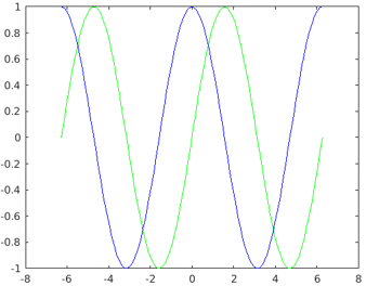
Explanation: Observe in the output that we have obtained our functions in the colors as expected.
Example #2 – 3 functions
Let us next take an example of 3 functions created in the same plot.
Syntax
Defining our functions:
X = linspace(-2*pi,2*pi)
a = sin (X)
b = cos (X)
c = X
- [Defining 100 equally distant points]
- [Defining our first function: sin function]
- [Defining our second function: cos function]
- [Defining our third function: a straight line]
Observe in the code that we have passed pre-defined color codes as arguments (Please refer to the table at the end of the article for pre-defined color codes)
How our input and output will look like in MATLAB console?
Code:
X = linspace(-2*pi,2*pi);
a = sin (X);
b = cos (X);
c = X
figure
plot(X, a, ‘g’, X, b, ‘b’, X, c, ‘y’)
Output:
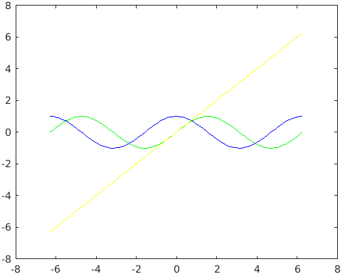
Explanation: As we can see in our output, we have got our functions in the colors as passed by us in the input.
How to Set the Color of Bar Plots?
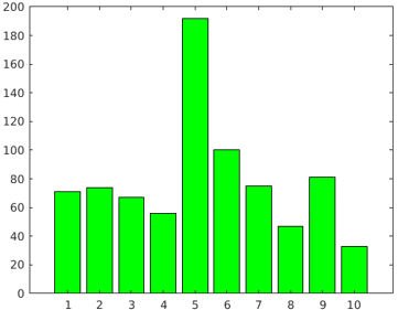
For this example, we will create a bar plot with bars of green color.
Syntax
Let us first define an array to create a Bar plot:
[71 746756 192 1007547 8133 ] bar (X, ‘g’)
- [Defining the array]
- [Plotting our bar plot]
Observe in the code that we have passed pre-defined color code for green as an argument (Please refer to the table at the end of the article for pre-defined color codes)
Code:
X = [71 74 67 56 192 100 75 47 81 33 ] bar (X, ‘g’
Output:
How to Set Color of Scatter Plots?
For this example, we will scatter plot of red color
Syntax:
a = linspace(0, 2*pi,100)
b = cos (a) + rand (1, 100)
scatter (a, b, ‘r’)
- [Defining 100 equally distant points]
- [Defining our cos function]
- [Plotting our scatter plot]
Observe in the code that we have passed pre-defined color code for red as an argument (Please refer to the table at the end of the article for pre-defined color codes)
Code:
a = linspace(0, 2*pi,100);
b = cos(a) + rand(1,100);
scatter(a, b, ‘r’)
Output:
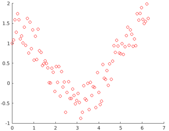
Observe in the output that we have obtained a scatter plot of red color, as passed by us in the input argument.
Conclusion
MATLAB can be used to plot our data for visualizing and intuitively understanding it. There could be instances when we have to plot multiple functions in a single plot, in such cases, colors become very handy to differentiate between different functions.
Recommended Articles
This is a guide to Matlab Plot Colors. Here we discuss an introduction to Matlab Plot Colors, along with color code table and respective examples. You can also go through our other related articles to learn more –
How to Plot MATLAB Graph with Colors, Markers and Line Specification?

Do you want to make you MATLAB plot more colorful and descriptive?
Earlier we have seen How to draw a Graph in MATLAB?. Those were a typical single color graph as shown below.
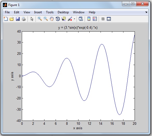
This graph still looks good as you are drawing a single graph on the MATLAB display.
Table of Contents
Why does everyone like to Plot MATLAB Graph with different Colors?
What if you are plotting multiple graphs on a single MATLAB display…
For plotting multiple graphs in a single window, it very difficult to distinguish one graph from another graph.
Let’s take an example.
You are plotting graphs for multiple mathematical equations like a sin wave, cos wave, exponential function on the same MATLAB display. After the running MATLAB program, you will get a number of graphs on the single MATLAB display. The end user will get more confused and will find it more difficult to understand and distinguish multiple graphs.
So you need to decorate each graph differently, like assigning a different color to each curve.
Each color describes one graph and that makes the graph self-descriptive.
How can you decorate your MATLAB graph?
In this tutorial, you will learn to plot the colorful graphs in MATLAB.
I am also explaining by plotting a graph for the mathematical equation on MATLAB R2013a by using a single color, simple marker and line specification.
We will also see what are the most important and useful color coding functions, marker style and line-specification designing functions available in MATLAB.
By using these functions, you can draw the graph or waveform as per your color and plotting style choice. And you can easily understand the particular equation’s graph.
Let’s begin by considering the top three essential components to decorate your graph more meaningful.
- Colour
- Marker Style
- Line Specification
Explanation of these three component functions are one-by-one,
MATLAB Plot Colors to draw the Graph
If you are drawing any picture on paper, you have different color pencils to use.
Likewise, for plotting the graph on MATLAB, we have different colors code or functions.
Widely, eight colors are used for MATLAB graph. And each color has the corresponding color code.
The below table shows color specification with the color code.
| Sr.No. | Colour Name | Colour Short Name | RGB Triplet | Hexadecimal Colour Code [Useful in MATLAB Program] |
| 1 | Black | k | [0 0 0] | ‘#000000’ |
| 2 | Blue | b | [0 0 1] | ‘#0000FF’ |
| 3 | Green | g | [0 1 0] | ‘#00FF00’ |
| 4 | Cyan | c | [0 1 1] | ‘#00FFFF’ |
| 5 | Red | r | [1 0 0] | ‘#FF0000’ |
| 6 | Magenta | m | [1 0 1] | ‘#FF00FF’ |
| 7 | Yellow | y | [1 1 0] | ‘#FFFF00’ |
| 8 | White | w | [1 1 1] | ‘#FFFFFF’ |
You can use these eight colors code to draw the colorful waveforms in MATLAB.
MATLAB Plot Marker | Different Style to Draw the Graph
Rather than just a simple line, do you want to make your waveform look different?
There are different marker style functions. For example, star format function, point format function, square format function, plus format function and so on.
In the below table, I am sharing the 12 marker style functions and its useful code for MATLAB graph.
How does the graph look different after using these marker styles? This we will see later in this tutorial example.
MATLAB Plot Line Specification | Code for MATLAB Graph
The four different spaceline codes are used for the plotting waveform or graph.
Check this blow table, for line specification code.
The syntax for plotting graph to add color, marker, and line specification:
These codes are placed inside single inverted comma.
Now its time to implement all three essentials components (color, marker, and line specifier) for decorating the MATLAB graph.
How to Plot MATLAB Graph with different colors, markers, and line specifier?
How to change Colour, Marker, and Line-Specification in MATLAB plot?
Let’s take these two mathematical equations to plot the MATLAB graph.
Solution:
The first mathematical equation is trigonometric.
And it’s derivative of a mathematical equation of y(x) is
MATLAB code:
Here is MATLAB code you can write to plot the graph for the function of f(x) and its d/dx (f(x)).
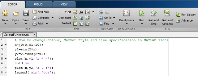
MATLAB PLot Colors code you can copy paste:
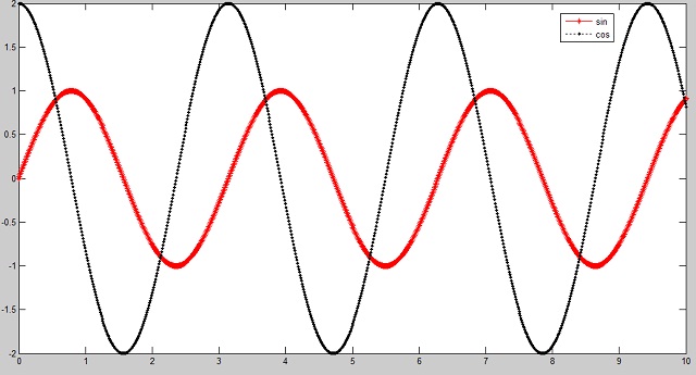
In this program, I have used the ‘legend’ function to label data series plotted on a graph. You can see in the below MATLAB output.
We are using different colors, markers and line specifications for plotting two different graphs.
MATLAB Output:
What’s Next:
I hope you learn to decorate our MATLAB graph with different colors, marker and line specifiers with the simple example of MATLAB graphs.
Now try MATLAB plot colors, marker styles and line specification on different MATLAB versions. Let’s make your graph more colorful.
Как менять цвет графика в матлаб

Syntax
Description
Vector and Matrix Data
plot( X , Y ) creates a 2-D line plot of the data in Y versus the corresponding values in X .
To plot a set of coordinates connected by line segments, specify X and Y as vectors of the same length.
To plot multiple sets of coordinates on the same set of axes, specify at least one of X or Y as a matrix.
plot( X , Y , LineSpec ) creates the plot using the specified line style, marker, and color.
plot( X 1, Y 1. X n, Y n) plots multiple pairs of x— and y-coordinates on the same set of axes. Use this syntax as an alternative to specifying coordinates as matrices.
plot( X 1, Y 1, LineSpec 1. X n, Y n, LineSpec n) assigns specific line styles, markers, and colors to each x—y pair. You can specify LineSpec for some x—y pairs and omit it for others. For example, plot(X1,Y1,»o»,X2,Y2) specifies markers for the first x—y pair but not for the second pair.
plot( Y ) plots Y against an implicit set of x-coordinates.
If Y is a vector, the x-coordinates range from 1 to length(Y) .
If Y is a matrix, the plot contains one line for each column in Y . The x-coordinates range from 1 to the number of rows in Y .
If Y contains complex numbers, MATLAB ® plots the imaginary part of Y versus the real part of Y . If you specify both X and Y , the imaginary part is ignored.
plot( Y , LineSpec ) plots Y using implicit x-coordinates, and specifies the line style, marker, and color.
Table Data
plot( tbl , xvar , yvar ) plots the variables xvar and yvar from the table tbl . To plot one data set, specify one variable for xvar and one variable for yvar . To plot multiple data sets, specify multiple variables for xvar , yvar , or both. If both arguments specify multiple variables, they must specify the same number of variables. (since R2022a)
plot( tbl , yvar ) plots the specified variable from the table against the row indices of the table. If the table is a timetable, the specified variable is plotted against the row times of the timetable. (since R2022a)
Additional Options
plot( ax , ___ ) displays the plot in the target axes. Specify the axes as the first argument in any of the previous syntaxes.
plot( ___ , Name,Value ) specifies Line properties using one or more name-value arguments. The properties apply to all the plotted lines. Specify the name-value arguments after all the arguments in any of the previous syntaxes. For a list of properties, see Line Properties .
p = plot( ___ ) returns a Line object or an array of Line objects. Use p to modify properties of the plot after creating it. For a list of properties, see Line Properties .
Examples
Create Line Plot
Create x as a vector of linearly spaced values between 0 and 2 π . Use an increment of π / 1 0 0 between the values. Create y as sine values of x . Create a line plot of the data.

Plot Multiple Lines
Define x as 100 linearly spaced values between — 2 π and 2 π . Define y1 and y2 as sine and cosine values of x . Create a line plot of both sets of data.

Create Line Plot From Matrix
Define Y as the 4-by-4 matrix returned by the magic function.
Create a 2-D line plot of Y . MATLAB® plots each matrix column as a separate line.

Specify Line Style
Plot three sine curves with a small phase shift between each line. Use the default line style for the first line. Specify a dashed line style for the second line and a dotted line style for the third line.

MATLAB® cycles the line color through the default color order.
Specify Line Style, Color, and Marker
Plot three sine curves with a small phase shift between each line. Use a green line with no markers for the first sine curve. Use a blue dashed line with circle markers for the second sine curve. Use only cyan star markers for the third sine curve.

Display Markers at Specific Data Points
Create a line plot and display markers at every fifth data point by specifying a marker symbol and setting the MarkerIndices property as a name-value pair.

Specify Line Width, Marker Size, and Marker Color
Create a line plot and use the LineSpec option to specify a dashed green line with square markers. Use Name,Value pairs to specify the line width, marker size, and marker colors. Set the marker edge color to blue and set the marker face color using an RGB color value.

Add Title and Axis Labels
Use the linspace function to define x as a vector of 150 values between 0 and 10. Define y as cosine values of x .
Create a 2-D line plot of the cosine curve. Change the line color to a shade of blue-green using an RGB color value. Add a title and axis labels to the graph using the title , xlabel , and ylabel functions.

Plot Durations and Specify Tick Format
Define t as seven linearly spaced duration values between 0 and 3 minutes. Plot random data and specify the format of the duration tick marks using the ‘DurationTickFormat’ name-value pair argument.

Plot Coordinates from a Table
A convenient way to plot data from a table is to pass the table to the plot function and specify the variables to plot.
Read weather.csv as a timetable tbl . Then display the first three rows of the table.
Plot the row times on the x -axis and the RainInchesPerMinute variable on the y -axis. When you plot data from a timetable, the row times are plotted on the x -axis by default. Thus, you do not need to specify the Time variable. Return the Line object as p . Notice that the axis labels match the variable names.
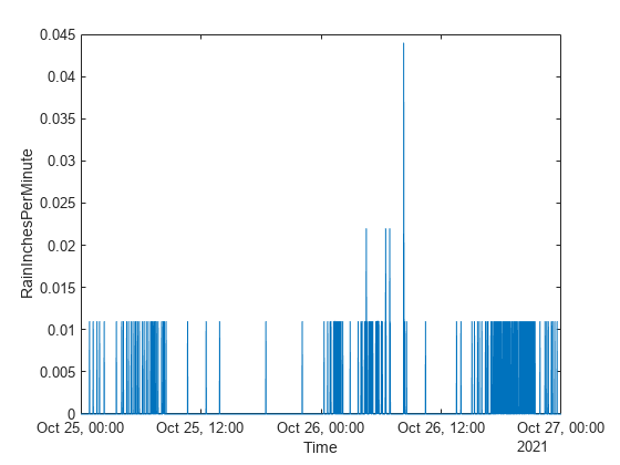
To modify aspects of the line, set the LineStyle , Color , and Marker properties on the Line object. For example, change the line to a red dotted line with point markers.

Plot Multiple Table Variables on One Axis
Read weather.csv as a timetable tbl , and display the first few rows of the table.
Plot the row times on the x -axis and the Temperature and PressureHg variables on the y -axis. When you plot data from a timetable, the row times are plotted on the x -axis by default. Thus, you do not need to specify the Time variable.
Add a legend. Notice that the legend labels match the variable names.

Specify Axes for Line Plot
Starting in R2019b, you can display a tiling of plots using the tiledlayout and nexttile functions. Call the tiledlayout function to create a 2-by-1 tiled chart layout. Call the nexttile function to create an axes object and return the object as ax1 . Create the top plot by passing ax1 to the plot function. Add a title and y -axis label to the plot by passing the axes to the title and ylabel functions. Repeat the process to create the bottom plot.

Modify Lines After Creation
Define x as 100 linearly spaced values between — 2 π and 2 π . Define y1 and y2 as sine and cosine values of x . Create a line plot of both sets of data and return the two chart lines in p .

Change the line width of the first line to 2. Add star markers to the second line. Use dot notation to set properties.

Plot Circle
Plot a circle centered at the point (4,3) with a radius equal to 2. Use axis equal to use equal data units along each coordinate direction.

Input Arguments
X — x-coordinates
scalar | vector | matrix
x-coordinates, specified as a scalar, vector, or matrix. The size and shape of X depends on the shape of your data and the type of plot you want to create. This table describes the most common situations.
Specify X and Y as scalars and include a marker. For example:
Specify X and Y as any combination of row or column vectors of the same length. For example:
Specify consecutive pairs of X and Y vectors. For example:
If all the sets share the same x— or y-coordinates, specify the shared coordinates as a vector and the other coordinates as a matrix. The length of the vector must match one of the dimensions of the matrix. For example:
Alternatively, specify X and Y as matrices of equal size. In this case, MATLAB plots each column of Y against the corresponding column of X . For example:
Data Types: single | double | int8 | int16 | int32 | int64 | uint8 | uint16 | uint32 | uint64 | categorical | datetime | duration
Y — y-coordinates
scalar | vector | matrix
y-coordinates, specified as a scalar, vector, or matrix. The size and shape of Y depends on the shape of your data and the type of plot you want to create. This table describes the most common situations.
Specify X and Y as scalars and include a marker. For example:
Specify X and Y as any combination of row or column vectors of the same length. For example:
Alternatively, specify just the y-coordinates. For example:
Specify consecutive pairs of X and Y vectors. For example:
If all the sets share the same x— or y-coordinates, specify the shared coordinates as a vector and the other coordinates as a matrix. The length of the vector must match one of the dimensions of the matrix. For example:
Alternatively, specify X and Y as matrices of equal size. In this case, MATLAB plots each column of Y against the corresponding column of X . For example:
Data Types: single | double | int8 | int16 | int32 | int64 | uint8 | uint16 | uint32 | uint64 | categorical | datetime | duration
LineSpec — Line style, marker, and color
string scalar | character vector
Line style, marker, and color, specified as a string scalar or character vector containing symbols. The symbols can appear in any order. You do not need to specify all three characteristics (line style, marker, and color). For example, if you omit the line style and specify the marker, then the plot shows only the marker and no line.
Example: «—or» is a red dashed line with circle markers.










tbl — Source table
table | timetable
Source table containing the data to plot, specified as a table or a timetable.
xvar — Table variables containing x-coordinates
string array | character vector | cell array | pattern | numeric scalar or vector | logical vector | vartype()
Table variables containing the x-coordinates, specified using one of the indexing schemes from the table.
A string, character vector, or cell array.
«A» or ‘A’ — A variable called A
[«A»,»B»] or <'A','B'>— Two variables called A and B
«Var»+digitsPattern(1) — Variables named «Var» followed by a single digit
An index number that refers to the location of a variable in the table.
A vector of numbers.
A logical vector. Typically, this vector is the same length as the number of variables, but you can omit trailing 0 or false values.
3 — The third variable from the table
[2 3] — The second and third variables from the table
[false false true] — The third variable
A vartype subscript that selects variables of a specified type.
vartype(«categorical») — All the variables containing categorical values
The table variables you specify can contain numeric, categorical, datetime, or duration values. If xvar and yvar both specify multiple variables, the number of variables must be the same.
Example: plot(tbl,[«x1″,»x2″],»y») specifies the table variables named x1 and x2 for the x-coordinates.
Example: plot(tbl,2,»y») specifies the second variable for the x-coordinates.
Example: plot(tbl,vartype(«numeric»),»y») specifies all numeric variables for the x-coordinates.
yvar — Table variables containing y-coordinates
string array | character vector | cell array | pattern | numeric scalar or vector | logical vector | vartype()
Table variables containing the y-coordinates, specified using one of the indexing schemes from the table.
A string, character vector, or cell array.
«A» or ‘A’ — A variable called A
[«A»,»B»] or <'A','B'>— Two variables called A and B
«Var»+digitsPattern(1) — Variables named «Var» followed by a single digit
An index number that refers to the location of a variable in the table.
A vector of numbers.
A logical vector. Typically, this vector is the same length as the number of variables, but you can omit trailing 0 or false values.
3 — The third variable from the table
[2 3] — The second and third variables from the table
[false false true] — The third variable
A vartype subscript that selects variables of a specified type.
vartype(«categorical») — All the variables containing categorical values
The table variables you specify can contain numeric, categorical, datetime, or duration values. If xvar and yvar both specify multiple variables, the number of variables must be the same.
Example: plot(tbl,»x»,[«y1″,»y2»]) specifies the table variables named y1 and y2 for the y-coordinates.
Example: plot(tbl,»x»,2) specifies the second variable for the y-coordinates.
Example: plot(tbl,»x»,vartype(«numeric»)) specifies all numeric variables for the y-coordinates.
ax — Target axes
Axes object | PolarAxes object | GeographicAxes object
Target axes, specified as an Axes object, a PolarAxes object, or a GeographicAxes object. If you do not specify the axes, MATLAB plots into the current axes or it creates an Axes object if one does not exist.
To create a polar plot or geographic plot, specify ax as a PolarAxes or GeographicAxes object. Alternatively, call the polarplot or geoplot function.
Name-Value Arguments
Specify optional pairs of arguments as Name1=Value1. NameN=ValueN , where Name is the argument name and Value is the corresponding value. Name-value arguments must appear after other arguments, but the order of the pairs does not matter.
Example: plot([0 1],[2 3],LineWidth=2)
Before R2021a, use commas to separate each name and value, and enclose Name in quotes.
Example: plot([0 1],[2 3],»LineWidth»,2)
Note
The properties listed here are only a subset. For a complete list, see Line Properties .
Color — Line color
[0 0.4470 0.7410] (default) | RGB triplet | hexadecimal color code | «r» | «g» | «b» | .
Line color, specified as an RGB triplet, a hexadecimal color code, a color name, or a short name.
For a custom color, specify an RGB triplet or a hexadecimal color code.
An RGB triplet is a three-element row vector whose elements specify the intensities of the red, green, and blue components of the color. The intensities must be in the range [0,1] , for example, [0.4 0.6 0.7] .
A hexadecimal color code is a string scalar or character vector that starts with a hash symbol ( # ) followed by three or six hexadecimal digits, which can range from 0 to F . The values are not case sensitive. Therefore, the color codes «#FF8800» , «#ff8800» , «#F80» , and «#f80» are equivalent.
Alternatively, you can specify some common colors by name. This table lists the named color options, the equivalent RGB triplets, and hexadecimal color codes.
Here are the RGB triplets and hexadecimal color codes for the default colors MATLAB uses in many types of plots.


Example: «blue»
Example: [0 0 1]
Example: «#0000FF»
LineStyle — Line style
«-» (default) | «—» | «:» | «-.» | «none»
Line style, specified as one of the options listed in this table.
LineWidth — Line width
0.5 (default) | positive value
Line width, specified as a positive value in points, where 1 point = 1/72 of an inch. If the line has markers, then the line width also affects the marker edges.
The line width cannot be thinner than the width of a pixel. If you set the line width to a value that is less than the width of a pixel on your system, the line displays as one pixel wide.
Marker — Marker symbol
«none» (default) | «o» | «+» | «*» | «.» | .
Marker symbol, specified as one of the values listed in this table. By default, the object does not display markers. Specifying a marker symbol adds markers at each data point or vertex.
MarkerIndices — Indices of data points at which to display markers
1:length(YData) (default) | vector of positive integers | scalar positive integer
Indices of data points at which to display markers, specified as a vector of positive integers. If you do not specify the indices, then MATLAB displays a marker at every data point.
Note
To see the markers, you must also specify a marker symbol.
Example: plot(x,y,»-o»,»MarkerIndices»,[1 5 10]) displays a circle marker at the first, fifth, and tenth data points.
Example: plot(x,y,»-x»,»MarkerIndices»,1:3:length(y)) displays a cross marker every three data points.
Example: plot(x,y,»Marker»,»square»,»MarkerIndices»,5) displays one square marker at the fifth data point.
MarkerEdgeColor — Marker outline color
«auto» (default) | RGB triplet | hexadecimal color code | «r» | «g» | «b» | .
Marker outline color, specified as «auto» , an RGB triplet, a hexadecimal color code, a color name, or a short name. The default value of «auto» uses the same color as the Color property.
For a custom color, specify an RGB triplet or a hexadecimal color code.
An RGB triplet is a three-element row vector whose elements specify the intensities of the red, green, and blue components of the color. The intensities must be in the range [0,1] , for example, [0.4 0.6 0.7] .
A hexadecimal color code is a string scalar or character vector that starts with a hash symbol ( # ) followed by three or six hexadecimal digits, which can range from 0 to F . The values are not case sensitive. Therefore, the color codes «#FF8800» , «#ff8800» , «#F80» , and «#f80» are equivalent.
Alternatively, you can specify some common colors by name. This table lists the named color options, the equivalent RGB triplets, and hexadecimal color codes.
Here are the RGB triplets and hexadecimal color codes for the default colors MATLAB uses in many types of plots.
MarkerFaceColor — Marker fill color
«none» (default) | «auto» | RGB triplet | hexadecimal color code | «r» | «g» | «b» | .
Marker fill color, specified as «auto» , an RGB triplet, a hexadecimal color code, a color name, or a short name. The «auto» option uses the same color as the Color property of the parent axes. If you specify «auto» and the axes plot box is invisible, the marker fill color is the color of the figure.
For a custom color, specify an RGB triplet or a hexadecimal color code.
An RGB triplet is a three-element row vector whose elements specify the intensities of the red, green, and blue components of the color. The intensities must be in the range [0,1] , for example, [0.4 0.6 0.7] .
A hexadecimal color code is a string scalar or character vector that starts with a hash symbol ( # ) followed by three or six hexadecimal digits, which can range from 0 to F . The values are not case sensitive. Therefore, the color codes «#FF8800» , «#ff8800» , «#F80» , and «#f80» are equivalent.
Alternatively, you can specify some common colors by name. This table lists the named color options, the equivalent RGB triplets, and hexadecimal color codes.
Here are the RGB triplets and hexadecimal color codes for the default colors MATLAB uses in many types of plots.
MarkerSize — Marker size
6 (default) | positive value
Marker size, specified as a positive value in points, where 1 point = 1/72 of an inch.
DatetimeTickFormat — Format for datetime tick labels
character vector | string
Format for datetime tick labels, specified as the comma-separated pair consisting of «DatetimeTickFormat» and a character vector or string containing a date format. Use the letters A-Z and a-z to construct a custom format. These letters correspond to the Unicode ® Locale Data Markup Language (LDML) standard for dates. You can include non-ASCII letter characters such as a hyphen, space, or colon to separate the fields.
If you do not specify a value for «DatetimeTickFormat» , then plot automatically optimizes and updates the tick labels based on the axis limits.
Example: «DatetimeTickFormat»,»eeee, MMMM d, yyyy HH:mm:ss» displays a date and time such as Saturday, April 19, 2014 21:41:06 .
The following table shows several common display formats and examples of the formatted output for the date, Saturday, April 19, 2014 at 9:41:06 PM in New York City.
| Value of DatetimeTickFormat | Example |
|---|---|
| «yyyy-MM-dd» | 2014-04-19 |
| «dd/MM/yyyy» | 19/04/2014 |
| «dd.MM.yyyy» | 19.04.2014 |
| «yyyy年 MM月 dd日» | 2014年 04月 19日 |
| «MMMM d, yyyy» | April 19, 2014 |
| «eeee, MMMM d, yyyy HH:mm:ss» | Saturday, April 19, 2014 21:41:06 |
| «MMMM d, yyyy HH:mm:ss Z» | April 19, 2014 21:41:06 -0400 |
For a complete list of valid letter identifiers, see the Format property for datetime arrays.
DatetimeTickFormat is not a chart line property. You must set the tick format using the name-value pair argument when creating a plot. Alternatively, set the format using the xtickformat and ytickformat functions.
The TickLabelFormat property of the datetime ruler stores the format.
DurationTickFormat — Format for duration tick labels
character vector | string
Format for duration tick labels, specified as the comma-separated pair consisting of «DurationTickFormat» and a character vector or string containing a duration format.
If you do not specify a value for «DurationTickFormat» , then plot automatically optimizes and updates the tick labels based on the axis limits.
To display a duration as a single number that includes a fractional part, for example, 1.234 hours, specify one of the values in this table.
| Value of DurationTickFormat | Description |
|---|---|
| «y» | Number of exact fixed-length years. A fixed-length year is equal to 365.2425 days. |
| «d» | Number of exact fixed-length days. A fixed-length day is equal to 24 hours. |
| «h» | Number of hours |
| «m» | Number of minutes |
| «s» | Number of seconds |
Example: «DurationTickFormat»,»d» displays duration values in terms of fixed-length days.
To display a duration in the form of a digital timer, specify one of these values.
In addition, you can display up to nine fractional second digits by appending up to nine S characters.
Example: «DurationTickFormat»,»hh:mm:ss.SSS» displays the milliseconds of a duration value to three digits.
DurationTickFormat is not a chart line property. You must set the tick format using the name-value pair argument when creating a plot. Alternatively, set the format using the xtickformat and ytickformat functions.
The TickLabelFormat property of the duration ruler stores the format.
Use NaN and Inf values to create breaks in the lines. For example, this code plots the first two elements, skips the third element, and draws another line using the last two elements:
plot uses colors and line styles based on the ColorOrder and LineStyleOrder properties of the axes. plot cycles through the colors with the first line style. Then, it cycles through the colors again with each additional line style.
You can change the colors and the line styles after plotting by setting the ColorOrder or LineStyleOrder properties on the axes. You can also call the colororder function to change the color order for all the axes in the figure. (since R2019b)
Документация

plot( X , Y ) создает 2D график данных в Y по сравнению с соответствующими значениями в X .
Чтобы построить набор координат, соединенных с методической точностью сегменты, задайте X и Y как векторы из той же длины.
Чтобы построить несколько наборов координат на том же наборе осей, задайте по крайней мере один из X или Y как матрица.
plot( X , Y , LineSpec ) создает график с помощью заданного стиля линии, маркера и цвета.
plot( X 1, Y 1. X n, Y n) графики несколько пар x — и y — координируют на том же наборе осей. Используйте этот синтаксис в качестве альтернативы определению координат как матрицы.
plot( X 1, Y 1, LineSpec 1. X n, Y n, LineSpec n) присваивает определенные стили линии, маркеры, и окрашивает к каждому x—y пару. Можно задать LineSpec для некоторого x—y пары и не используют его для других. Например, plot(X1,Y1,’o’,X2,Y2) задает маркеры для первого x—y пара, но не для второй пары.
plot( Y ) графики Y против неявного набора x — координаты.
Если Y вектор, x — диапазон координат от 1 до length(Y) .
Если Y матрица, график содержит одну линию для каждого столбца в Y . x — координирует диапазон от 1 до количества строк в Y .
Если Y содержит комплексные числа, MATLAB ® строит мнимую часть Y по сравнению с действительной частью Y . Если вы задаете оба X и Y , мнимая часть проигнорирована.
plot( Y , LineSpec ) задает стиль линии, маркер и цвет.
plot( ___ , Name,Value ) задает Line свойства с помощью одних или нескольких аргументов name-value. Свойства применяются ко всем построенным линиям. Задайте аргументы name-value после всех аргументов в любом из предыдущих синтаксисов. Для списка свойств смотрите Line Properties .
plot( ax , ___ ) отображает график в целевых осях. Задайте оси в качестве первого аргумента в любом из предыдущих синтаксисов.
p = plot( ___ ) возвращает Line возразите или массив Line объекты. Используйте p изменить свойства графика после создания его. Для списка свойств смотрите Line Properties .
Примеры
Построение графика
Создайте x как вектор из линейно распределенных значений между 0 и 2 π . Используйте шаг π / 1 0 0 между значениями. Создайте y как значения синуса x . Постройте график данных.

Построение нескольких графиков
Задайте x как 100 линейно распределенных значений между — 2 π и 2 π . Задайте y1 и y2 как синус и значения косинуса x Создать график для обоих наборов данных.

Построение графика из матрицы
Задайте Y как матрица 4 на 4, возвращенная magic функция.
Постройте 2D график для данных Y MATLAB® строит график для каждого столбца матрицы как новый график, новой линией.

Определение стиля линии
Постройте три синусоиды с маленьким сдвигом фазы между каждой линией. Используйте стиль линии по умолчанию для первой линии. Задайте стиль пунктирной линии для второй линии и стиль точечной линии для третьей линии.

MATLAB® циклически повторяет цвет линии через порядок цвета по умолчанию.
Определение стиля линии, цвета и маркера
Постройте три синусоиды с маленьким сдвигом фазы между каждой линией. Используйте зеленую линию без маркеров для первой синусоиды. Используйте синюю пунктирную линию с круговыми маркерами для второй синусоиды. Используйте только голубые маркеры-звездочки для третьей синусоиды.

Отображение маркеров в определенных точках данных
Постройте график и маркеры отображения в каждой пятой точке данных путем определения символа маркера и установки MarkerIndices свойство как пара "имя-значение".

Определение ширины линии, размера маркера и цвета маркера
Постройте график и используйте LineSpec опция, чтобы задать пунктирную зеленую линию с квадратными маркерами. Используйте Name,Value пары, чтобы задать ширину линии, размер маркера и цвета маркера. Установите цвет обводки маркера на синий и выберите цвет поверхности маркера с помощью значения цвета RGB.

Добавление заголовка и подписей по осям
Используйте linspace функция, чтобы задать x как вектор из 150 значений между 0 и 10. Задайте y как значения косинуса x .
Создайте 2D график косинусоиды. Измените цвет линии в оттенок сине-зеленого использования значения цвета RGB. Добавьте заголовок и подписи по осям к графику с помощью title xlabel , и ylabel функции.

Графическое изображение длительности и определение формата метки деления
Задайте t как семь линейно расположил с интервалами duration значения между 0 и 3 минутами. Отобразите случайные данные на графике и задайте формат duration отметки деления с помощью ‘DurationTickFormat’ аргумент пары "имя-значение".

Задание осей для графика
Начиная в R2019b, можно отобразить плиточное размещение графиков с помощью tiledlayout и nexttile функции. Вызовите tiledlayout функция, чтобы создать 2 1 мозаичное размещение графика. Вызовите nexttile функция, чтобы создать объект осей и возвратить объект как ax1 . Создайте главный график путем передачи ax1 к plot функция. Добавьте заголовок и метку оси Y к графику путем передачи осей title и ylabel функции. Повторите процесс, чтобы создать нижний график.

Изменение линни после ее создания
Задайте x как 100 линейно распределенных значений между — 2 π и 2 π . Задайте y1 и y2 как синус и значения косинуса x . Постройте график обоих наборов данных и возвратите эти две линии на графике в p .

Измените ширину первой линни, задав значение 2. Добавьте маркеры-звездочки во вторую линию. Используйте запись через точку, чтобы установить свойства.

Рисование окружности
Постройте круг, сосредоточенный в точке (4,3) с радиусом, равным 2. Используйте axis equal для задания одинаковых маштабов по осям.

Входные параметры
X — x — координаты
скаляр | вектор | матрица
x- в виде скаляра, вектора или матрицы. Размер и форма X зависит от формы ваших данных и типа графика, который вы хотите создать. Эта таблица описывает наиболее распространенные ситуации.
Задайте X и Y как скаляры и включают маркер. Например:
Задайте X и Y как любая комбинация строки или вектор-столбцы той же длины. Например:
Задайте последовательные пары X и Y векторы. Например:
Если все наборы совместно используют тот же x — или y — координаты, задают разделяемые координаты как вектор и другие координаты как матрица. Длина вектора должна совпадать с одной из размерностей матрицы. Например:
В качестве альтернативы задайте X и Y как матрицы равного размера. В этом случае, графики MATLAB каждый столбец Y против соответствующего столбца X . Например:
Типы данных: single | double | int8 | int16 | int32 | int64 | uint8 | uint16 | uint32 | uint64 | categorical | datetime | duration
Y — y — координаты
скаляр | вектор | матрица
y- в виде скаляра, вектора или матрицы. Размер и форма Y зависит от формы ваших данных и типа графика, который вы хотите создать. Эта таблица описывает наиболее распространенные ситуации.
Задайте X и Y как скаляры и включают маркер. Например:
Задайте X и Y как любая комбинация строки или вектор-столбцы той же длины. Например:
В качестве альтернативы задайте только y — координаты. Например:
Задайте последовательные пары X и Y векторы. Например:
Если все наборы совместно используют тот же x — или y — координаты, задают разделяемые координаты как вектор и другие координаты как матрица. Длина вектора должна совпадать с одной из размерностей матрицы. Например:
В качестве альтернативы задайте X и Y как матрицы равного размера. В этом случае, графики MATLAB каждый столбец Y против соответствующего столбца X . Например:
Типы данных: single | double | int8 | int16 | int32 | int64 | uint8 | uint16 | uint32 | uint64 | categorical | datetime | duration
LineSpec — Стиль линии, маркер и цвет
вектор символов | строка
Стиль линии, цвет и маркер задается как символ или строка символов. Символы могут появиться в любом порядке. Вы не должны задавать все три характеристики (стиль линии, маркер и цвет). Например, если вы не используете стиль линии и задаете маркер, затем график показывает только маркер и никакую линию.
Пример: ‘—or’ красная пунктирная линия с круговыми маркерами










ax — Целевые оси
Axes возразите | PolarAxes возразите | GeographicAxes объект
Целевые оси в виде Axes объект, PolarAxes объект или GeographicAxes объект. Если вы не задаете оси, графики MATLAB в текущую систему координат, или это создает Axes возразите, не существуете ли вы.
Чтобы создать полярный график или географический график, задайте ax как PolarAxes или GeographicAxes объект. В качестве альтернативы вызовите polarplot или geoplot функция.
Аргументы name-value
Задайте дополнительные разделенные запятой пары Name,Value аргументы. Name имя аргумента и Value соответствующее значение. Name должен появиться в кавычках. Вы можете задать несколько аргументов в виде пар имен и значений в любом порядке, например: Name1, Value1, . NameN, ValueN .
Пример: ‘Marker’,’o’,’MarkerFaceColor’,’red’
Свойства линии на графике, перечисленные здесь, являются только подмножеством. Для полного списка смотрите Line Properties .
Color ‘LineColor’
[0 0.4470 0.7410] (значение по умолчанию) | триплет RGB | шестнадцатеричный цветовой код | ‘r’ | ‘g’ | ‘b’ | .
Цвет линии в виде триплета RGB, шестнадцатеричного цветового кода, названия цвета или краткого названия.
Для пользовательского цвета задайте триплет RGB или шестнадцатеричный цветовой код.
Триплет RGB представляет собой трехэлементный вектор-строку, элементы которого определяют интенсивность красных, зеленых и синих компонентов цвета. Интенсивность должна быть в области значений [0,1] ; например, [0.4 0.6 0.7] .
Шестнадцатеричный цветовой код является вектором символов или строковым скаляром, который запускается с символа хеша ( # ) сопровождаемый тремя или шестью шестнадцатеричными цифрами, которые могут лежать в диапазоне от 0 к F . Значения не являются чувствительными к регистру. Таким образом, цветовые коды ‘#FF8800’ , ‘#ff8800’ , ‘#F80’ , и ‘#f80’ эквивалентны.
Кроме того, вы можете задать имена некоторых простых цветов. Эта таблица приводит опции именованного цвета, эквивалентные триплеты RGB и шестнадцатеричные цветовые коды.
Вот являются триплеты RGB и шестнадцатеричные цветовые коды для цветов по умолчанию использованием MATLAB во многих типах графиков.







Пример: ‘blue’
Пример: [0 0 1]
Пример: ‘#0000FF’
LineStyle — Стиль линии
‘-‘ (значение по умолчанию) | ‘—‘ | ‘:’ | ‘-.’ | ‘none’
Стиль линии в виде одной из опций перечислен в этой таблице.
LineWidth ‘LineWidth’
0.5 (значение по умолчанию) | положительное значение
Ширина линии в виде положительного значения в точках, где 1 точка = 1/72 дюйма. Если у линии есть маркеры, ширина линии также влияет на края маркера.
Ширина линии не может быть более тонкой, чем ширина пикселя. Если вы устанавливаете ширину линии на значение, которое меньше ширины пикселя в вашей системе, отображения линии как один пиксель шириной.
Marker — Символ маркера
‘none’ (значение по умолчанию) | ‘o’ | ‘+’ | ‘*’ | ‘.’ | .
Символ маркера в виде одного из значений перечислен в этой таблице. По умолчанию объект не отображает маркеры. Определение символа маркера добавляет маркеры в каждой точке данных или вершине.
MarkerIndices — Индексы точек данных, в которых можно отобразить маркеры
1:length(YData) (значение по умолчанию) | вектор из положительных целых чисел | скалярное положительное целое число
Индексы точек данных, в которых можно отобразить маркеры в виде вектора из положительных целых чисел. Если вы не задаете индексы, то MATLAB отображает маркер в каждой точке данных.
Примечание
Чтобы видеть маркеры, необходимо также задать символ маркера.
Пример: plot(x,y,’-o’,’MarkerIndices’,[1 5 10]) отображает круговой маркер во-первых, пятые, и десятые точки данных.
Пример: plot(x,y,’-x’,’MarkerIndices’,1:3:length(y)) отображает перекрестный маркер каждые три точки данных.
Пример: plot(x,y,’Marker’,’square’,’MarkerIndices’,5) отображения один квадратный маркер в пятой точке данных.
MarkerEdgeColor — Цвет контура маркера
‘auto’ (значение по умолчанию) | триплет RGB | шестнадцатеричный цветовой код | ‘r’ | ‘g’ | ‘b’ | .
Цвет контура маркера в виде ‘auto’ , триплет RGB, шестнадцатеричный цветовой код, название цвета или краткое название. Значение по умолчанию ‘auto’ использует тот же цвет в качестве Color свойство.
Для пользовательского цвета задайте триплет RGB или шестнадцатеричный цветовой код.
Триплет RGB представляет собой трехэлементный вектор-строку, элементы которого определяют интенсивность красных, зеленых и синих компонентов цвета. Интенсивность должна быть в области значений [0,1] ; например, [0.4 0.6 0.7] .
Шестнадцатеричный цветовой код является вектором символов или строковым скаляром, который запускается с символа хеша ( # ) сопровождаемый тремя или шестью шестнадцатеричными цифрами, которые могут лежать в диапазоне от 0 к F . Значения не являются чувствительными к регистру. Таким образом, цветовые коды ‘#FF8800’ , ‘#ff8800’ , ‘#F80’ , и ‘#f80’ эквивалентны.
Кроме того, вы можете задать имена некоторых простых цветов. Эта таблица приводит опции именованного цвета, эквивалентные триплеты RGB и шестнадцатеричные цветовые коды.
Вот являются триплеты RGB и шестнадцатеричные цветовые коды для цветов по умолчанию использованием MATLAB во многих типах графиков.
MarkerFaceColor — Цвет заливки маркера
‘none’ (значение по умолчанию) | ‘auto’ | Триплет RGB | шестнадцатеричный цветовой код | ‘r’ | ‘g’ | ‘b’ | .
Цвет заливки маркера в виде ‘auto’ , триплет RGB, шестнадцатеричный цветовой код, название цвета или краткое название. ‘auto’ опция использует тот же цвет в качестве Color свойство родительских осей. Если вы задаете ‘auto’ и поле графика осей невидимо, цвет заливки маркера является цветом фигуры.
Для пользовательского цвета задайте триплет RGB или шестнадцатеричный цветовой код.
Триплет RGB представляет собой трехэлементный вектор-строку, элементы которого определяют интенсивность красных, зеленых и синих компонентов цвета. Интенсивность должна быть в области значений [0,1] ; например, [0.4 0.6 0.7] .
Шестнадцатеричный цветовой код является вектором символов или строковым скаляром, который запускается с символа хеша ( # ) сопровождаемый тремя или шестью шестнадцатеричными цифрами, которые могут лежать в диапазоне от 0 к F . Значения не являются чувствительными к регистру. Таким образом, цветовые коды ‘#FF8800’ , ‘#ff8800’ , ‘#F80’ , и ‘#f80’ эквивалентны.
Кроме того, вы можете задать имена некоторых простых цветов. Эта таблица приводит опции именованного цвета, эквивалентные триплеты RGB и шестнадцатеричные цветовые коды.
Вот являются триплеты RGB и шестнадцатеричные цветовые коды для цветов по умолчанию использованием MATLAB во многих типах графиков.
MarkerSize ‘MarkerSize’
6 (значение по умолчанию) | положительное значение
Размер маркера в виде положительного значения в точках, где 1 точка = 1/72 дюйма.
DatetimeTickFormat — Формат для datetime метки в виде галочки
вектор символов | строка
Формат для datetime метки в виде галочки в виде разделенной запятой пары, состоящей из ‘DatetimeTickFormat’ и вектор символов или строка, содержащая формат даты. Используйте буквы A-Z и a-z создать пользовательский формат. Эти буквы соответствуют Unicode ® Стандарт языка разметки данных локали (LDML) для дат. Можно включать символы буквы non-ASCII, такие как дефис, пробел или двоеточие, чтобы разделить поля.
Если вы не задаете значение для ‘DatetimeTickFormat’ то plot автоматически оптимизирует и обновляет метки в виде галочки на основе пределов по осям.
Пример: ‘DatetimeTickFormat’,’eeee, MMMM d, yyyy HH:mm:ss’ отображает дату и время, такую как Saturday, April 19, 2014 21:41:06 .
Следующая таблица показывает несколько общих форматов отображения и примеров отформатированного вывода для даты, суббота, 19 апреля 2014 в 21:41:06 в Нью-Йорке.
| Значение DatetimeTickFormat | Пример |
|---|---|
| ‘yyyy-MM-dd’ | 2014-04-19 |
| ‘dd/MM/yyyy’ | 19/04/2014 |
| ‘dd.MM.yyyy’ | 19.04.2014 |
| ‘yyyy年 MM月 dd日’ | 2014年 04月 19日 |
| ‘MMMM d, yyyy’ | April 19, 2014 |
| ‘eeee, MMMM d, yyyy HH:mm:ss’ | Saturday, April 19, 2014 21:41:06 |
| ‘MMMM d, yyyy HH:mm:ss Z’ | April 19, 2014 21:41:06 -0400 |
Для полного списка допустимых идентификаторов буквы смотрите Format свойство для массивов datetime.
DatetimeTickFormat не свойство линии на графике. Необходимо установить формат метки деления с помощью аргумента пары "имя-значение" при создании графика. В качестве альтернативы установите формат с помощью xtickformat и ytickformat функции.
TickLabelFormat свойство линейки datetime хранит формат.
DurationTickFormat — Формат для duration метки в виде галочки
вектор символов | строка
Формат для duration метки в виде галочки в виде разделенной запятой пары, состоящей из ‘DurationTickFormat’ и вектор символов или строка, содержащая формат длительности.
Если вы не задаете значение для ‘DurationTickFormat’ то plot автоматически оптимизирует и обновляет метки в виде галочки на основе пределов по осям.
Чтобы отобразить длительность как, один номер, который включает дробную часть, например, 1,234 часа, задает одно из значений в этой таблице.
| Значение DurationTickFormat | Описание |
|---|---|
| ‘y’ | Номер точных лет фиксированной длины. Год фиксированной длины равен 365,2425 дням. |
| ‘d’ | Номер точных дней фиксированной длины. День фиксированной длины равен 24 часам. |
| ‘h’ | Номер часов |
| ‘m’ | Номер минут |
| ‘s’ | Номер секунд |
Пример: ‘DurationTickFormat’,’d’ значения длительности отображений в терминах дней фиксированной длины.
Чтобы отобразить длительность в форме цифрового таймера, задайте одно из этих значений.
Кроме того, можно отобразить до девяти цифр доли секунды путем добавления до девяти S ‘characters’.
Пример: ‘DurationTickFormat’,’hh:mm:ss.SSS’ отображает миллисекунды значения длительности к трем цифрам.
DurationTickFormat не свойство линии на графике. Необходимо установить формат метки деления с помощью аргумента пары "имя-значение" при создании графика. В качестве альтернативы установите формат с помощью xtickformat и ytickformat функции.
TickLabelFormat свойство линейки длительности хранит формат.
Советы
Используйте NaN и Inf специальные символы, чтобы создать пропуски на линии графика. Например, этот код строит первые два элемента, пропускает третий элемент и проводит другую линию с помощью последних двух элементов:
plot цвета использования и стили линии на основе ColorOrder и LineStyleOrder свойства осей. plot циклы через цвета с первым стилем линии. Затем это циклически повторяется через цвета снова с каждым дополнительным стилем линии.
Начиная в R2019b, можно изменить цвета и стили линии после графического вывода путем установки ColorOrder или LineStyleOrder свойства на осях. Можно также вызвать colororder функционируйте, чтобы изменить последовательность цветов для всех осей на рисунке.