Using DB Browser for SQLite
In Windows the installation of DB Browser does not create a desktop icon. To explicitly launch the application after installing it, use the windows button (bottom left of screen) and type in ‘DB Browser’ in the search bar and selecting the application when it appears.
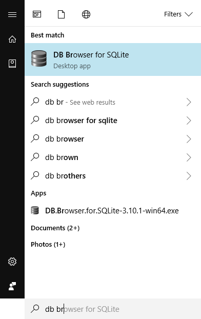
For Mac users, launch the spotlight search bar (press “command” + the space bar on your keyboard) and enter ‘DB Browser.’ Select the application when it appears.

The Initial screen
The initial screen of DB Browser will look something like this, the panes may be in a different configuration;
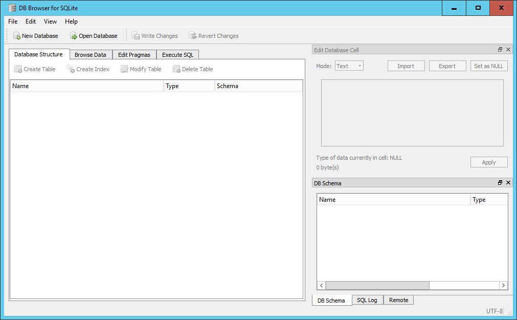
A small menu system consisting of File, Edit, View and Help. Below the menu system is a toolbar with four options; New Database, Open Database, Write Changes and Revert Changes. Below the toolbar is a 4-tabbed pane for; Database Structure, Browse Data, Edit Pragmas and Execute SQL. Initially these will be quite empty as we haven’t created or opened a database yet. In general we will see how each of these are used as we go through the lesson with the exception of the Edit Pragmas tab which deals with system wide parameters which we won’t want to change.
On the right hand side there are two further panes, at the top is the Edit Database Cell pane which is grayed out. Below it is a 3-tabbed pane for DB Schema, SQL log and Remote. We are only really interested in the DB Schema tab.
Initial changes to the layout.
The overall layout of DB Browser is quite flexible. The panes on the right-hand side can be dragged and dropped into any position, the individual tabs on the bottom pane closed directly from the pane and re-opened from the menu View item.
We will make a couple of initial changes to the layout of the screen. These will be retained across sessions.
- From the View menu item un-select the ‘Edit Database Cell’ icon to the left of the text. This will make the pane close and the bottom pane will be expanded automatically to fill the space.
- a) On Windows, From the ViewEdit menu item select ‘preferences’ and select the Data Browser tab.
- b) On Mac, From the “DB Browser for SQLite” menu item select ‘preferences’ and select the Data Browser tab.
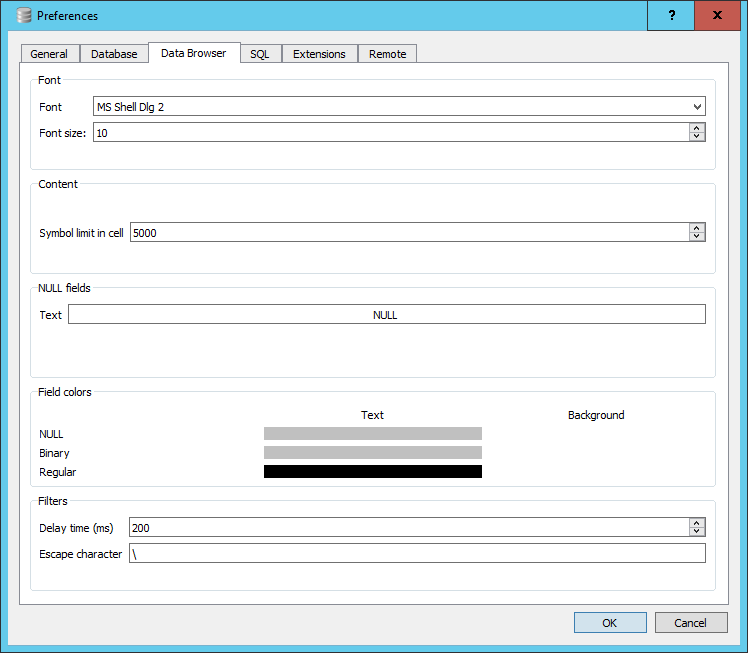
Towards the bottom there is a section dealing with Field colors. You will see three bars below the word Text, to the right there are in fact three invisible bars for the Background. Click in the area for the Background color for NULL. A colour selector window will open, select Red. The bar will turn Red. This is now the default background cell colour that will be used to display NULL values in you tables. We will discuss the meaning of NULL values in a table in a later episode.
You can now close the preference window by clicking OK.
Opening a database
One of the datasets we will be using this lesson is the SQL_SAFI database, a sample of a farm survey. If you do not already have a copy of this database you can download it from here.
To open the database in DB Browser do the following;
- Click on the ‘open database’ button in the toolbar.
- Navigate to where you have stored the database file on your local machine, select it and click open.
When you open the database, the ‘Database Structure’ tab on the left and the ‘DB Schema’ pane on the right will look very similar. However the ‘DB Schema’ pane is only there to allow you to see the details of the schema for the tables. In particular what tables are in the database and the fields and their types which are in each table.
The ‘Database Structure’ tab on the left allows you to initiate actions on the tables. If you right click on a table name in the ‘DB Schema’ pane, nothing happens. However, if you do the same in the ‘Database Structure’ menu you will be given a set of possible actions. These are the same actions that are available from the toolbar at the top of the tab.
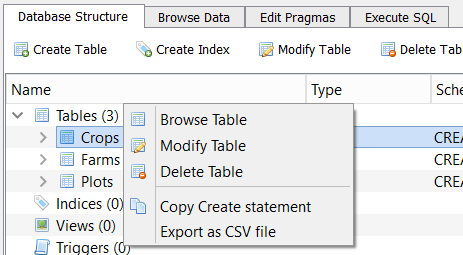
If you select ‘Browse Table’, the data from the table is loaded into the ‘Browse Data’ pane from where it can be examined or filtered. You can also select the table you wish to Browse directly from here.
There are options for ‘New Record’ and ‘Delete Record’. As our interest is in analysing existing data not creating or deleting data, it is unlikely that you will want to use these options.
Running SQL Queries
We will be running queries extensively in future episodes. For now we will just provide an outline of the environment.
In the left hand pane if you select the Execute SQL tab, you will be presented with a three paned window and a small toolbar. The top pane is itself tabbed with the initial tab labeled ‘SQL 1’. This is the SQL editor pane into which you will type your queries.
Below is a simple example query and the results.
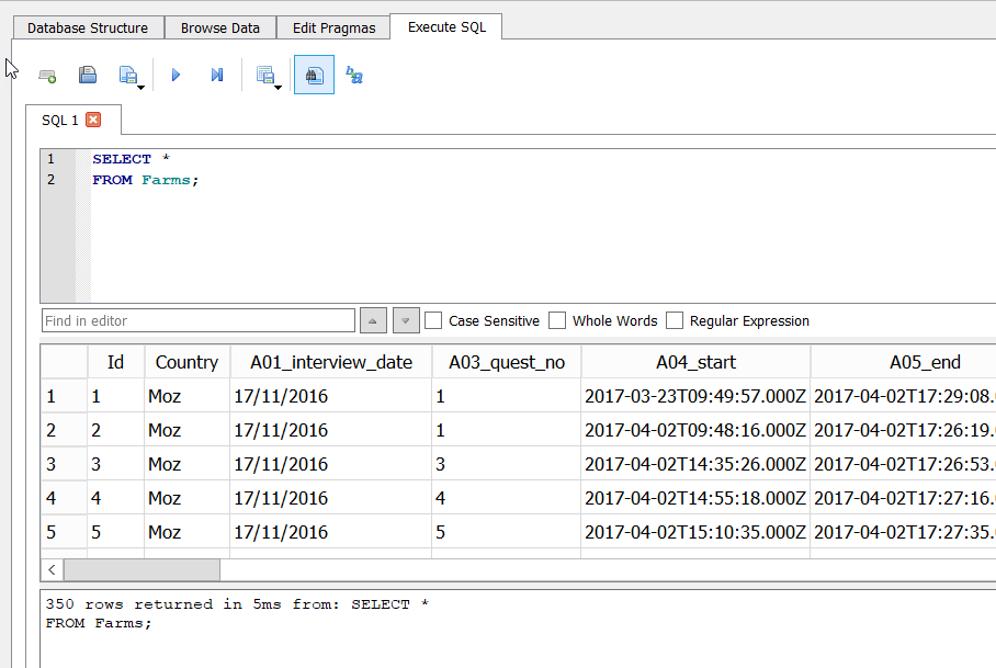
Notice that the query has been written over multiple lines. This is commonly done to aid readability. The second pane has the tabular results, and the bottom pane has a message indicating how many rows were returned, how long it took and a copy of the SQL statement that was executed.
On the toolbar at the top there are eight buttons. Left to right they are:
- Open Tab (creates a new tab in the editor)
- Open SQL file (allows you to load a prepared file of SQL into the editor — the tab takes the name of he file)
- Save SQL file (allows you to save the current contents of the active pane to the local file system)
- Execute SQL (Executes all of the SQL statements in the editor pane)
- Execute current line (Actually executes whatever is selected)
- Save Results (Either to a CSV file or as a database view. We will look at views in a later episode)
- Find (Text in the editor window)
- Find & Replace (Text in the editor window)
Because it is possible to have and execute multiple SQL statements in the same editor pane, each must be terminated with a ‘;’. If you only have a single statement you don’t need it, but it might be considered best practice to always include it.
The pane below the editor is the Results pane. The results of running your query will appear here in a simple tabular format. The bottom pane is for messages about the execution, either an error message or an indication of how many rows were returned by the query.
Explore another Table
-
1. What would be the SQL query to select all the entries from «crops_rice_old»? 2. How many entries are in the «crops_rice_old» table? 3. What information do you think «Plot_Id» represents?
Solution
Creating a database
As well as opening (connecting) to existing databases it is also possible to create new SQLite databases and tables using DB Browser. To create a database click the New Database button from the main toolbar (also available from the File menu). You will initially be asked for a name for the database and where you want to save it. It is saved as a single file. You can choose your own extension but ‘sqlite’ is recommended. If you do not provide a default, then a ‘.db’ extension will be used. Although the new database is empty, in that there are no tables in it, the .sqlite file itself is not empty.
Once you have saved the database file the Create Table wizard will open allowing you to create a table. You can cancel this as we will be going through the create table process in a later episode.
Write Changes & Revert Changes
Much of our SQL work involves looking at existing data using SQL queries and possibly writing out the results to a CSV file, in general we will not be changing the contents of the database.
However if, during your DB Browser session, you were to create or delete a table or create a view, then the changes are not automatically written to the database file.
Создание SQLite базы данных в DB Browser for SQLite

Базы данных SQLite очень удобны для работы с небольшими объемами данных как в Windows приложениях, так и в Android приложениях. В статье говорится, как создавать и подготавливать базы данных заранее.
Особенно SQLite удобен тем, что не нужно поднимать сервер СУБД перед использованием в приложениях.
Установка DB Browser for SQLite
Итак, скачиваем версию без установщика DB Browser for SQLite ( SQLiteBrowser ): http://sqlitebrowser.org:

Просто распаковываем архив. В нем будет два EXE файла:

Файл DB Browser for SQLite.exe представляет обычную версию программы, а файл DB Browser for SQLCipher.exe позволяет работать с зашифрованными базами данных. И во второй программе есть вот такой пункт:


Создание базы данных
Создадим простую базу данных database с одной таблицей и тремя столбцами:


Появится окно создания таблицы в программе:

Создадим таблицу People :

Ввиду того, что вдруг база данных будет использоваться в Android, то первым полем задавайте идентификатор по имени _id :

Добавим, например, поля Name и Age :


Во вкладке Данные можем вносить данные:


У вас есть готовая база данных SQLite, которую можете использовать, где вам нужно:

Статья обновлена 2019-08-05
- SQLite
- Базы данных
- blog
- it
- programming
Базы данных SQLite очень удобны для работы с небольшими объемами данных как в Windows приложениях, так и в Android приложениях. В статье говорится, как создавать и подготавливать базы данных заранее.
Базы данных SQLite очень удобны для работы с небольшими объемами данных как в Windows приложениях, так и в Android приложениях. В статье говорится, как создавать и подготавливать базы данных заранее.
Takeaways
Congrats! If you made it here, you now have a pretty good idea of how to use SQLite Browser. This page is also a great reference to keep handy in case you forget how to do something like change the data type, or import tables.
Filed under: SQL by Boxplot Analytics
No Comments »
Understanding JOINs in SQL
Joins in SQL
Joins are one of the most important (if not THE most important) concepts in SQL. If you take the time to solidly understand how joins work, you’ll be in an excellent place for writing queries. So, let’s dive in!
Join Definitions
Joining tables in SQL is a way of combining them. It is directly comparable to a VLOOKUP in Excel, so if you are familiar wtih VLOOKUPs you already understand how joins work. For example, let’s say you have a table that contains orders placed by your customers (each row in that table represents a unique order). Then you have a second table that is only items that have been returned by your customers (each row in that table represents a unique order too, but not all orders are returned so the table has fewer rows).
Orders Table
| order_id | product | cost_per_unit | total_amount | profit | shipping_method |
|---|---|---|---|---|---|
| 1 | A | 5 | 70 | 5 | Air |
| 2 | B | 10 | 120 | 97 | Air |
| 3 | C | 15 | 150 | 135 | Air |
| 4 | A | 5 | 20 | 10 | Air |
| 5 | B | 10 | 110 | 96 | Air |
| 6 | C | 15 | 30 | 5 | Air |
| 7 | A | 5 | 45 | 9 | Air |
| 8 | B | 10 | 150 | 64 | Air |
| 9 | C | 15 | 210 | 63 | Air |
| 10 | A | 5 | 65 | 44 | Air |
| 11 | B | 10 | 120 | 76 | Air |
| 12 | C | 15 | 30 | 18 | Air |
| 13 | A | 5 | 20 | 19 | Ground |
| 14 | B | 10 | 100 | 59 | Ground |
| 15 | C | 15 | 30 | 14 | Ground |
| 16 | A | 5 | 55 | 15 | Ground |
| 17 | B | 10 | 10 | 1 | Ground |
| 18 | C | 15 | 105 | 28 | Ground |
| 19 | A | 5 | 75 | 37 | Ground |
| 20 | B | 10 | 50 | 41 | Ground |
| 21 | C | 15 | 15 | 9 | Ground |
| 22 | A | 5 | 30 | 22 | Ground |
| 23 | B | 10 | 120 | 117 | Ground |
| 24 | C | 15 | 195 | 166 | Ground |
| 25 | A | 5 | 20 | 1 | Ground |
Returns Table
| id | amount_returned | Reason |
|---|---|---|
| 15 | 10 | Broken |
| 2 | 115 | No Reason Given |
| 24 | 85 | Unsatisfied |
| 7 | 15 | Unsatisfied |
| 12 | 20 | Unsatisfied |
| 9 | 130 | Unsatisfied |
| 17 | 10 | No Reason Given |
| 21 | 15 | No Reason Given |
| 18 | 70 | Broken |
| 17 | 10 | Broken |
You can’t just copy and paste these tables next to each other to figure out what was returned, because the rows won’t match up. You need a way of comparing each row in the orders table to the returns table to see if a match exists, and then bring back the information from the returns table that you’re interested in. Enter joins!
Let’s take a look at join syntax first:
Notice the ON statement, which is required for every join. You need to pick a column from each table that you want SQL to compare in order to join them together, and that’s what the ON statement is specifying. This example says compare the id column in table_1 to the id column in table_2 when trying to match up rows between the two tables during the join.
How do you choose which colunns to use for the ON statement? Generally you want to pick a column that uniquely identifies each row, like an id number. The two columns don’t have to have the exact same name, but they need to be the same type (for example, integer or text) and represent the same thing. The order_id columnn from the orders table above is the same thing as the id column in the returns table – they both represent the id of the order.
There are four types of joins: left, right, inner and outer. The right join functionally does the same thing as the left join, so many SQL programs are choosing not even to support it anymore. For that reason, we won’t be covering it in this article.
As usual, we’ll start with a basic example. Say you have a database with the following two tables in it:
nutrition1
| id | name | calcium | serving_size | weight |
|---|---|---|---|---|
| 1 | apples | 10 | 1 ea | 138 |
| 2 | asparagus | 22 | 1/2 cup | 90 |
| 3 | avocado | 19 | 1 ea | 173 |
| 4 | bamboo shoots | 10 | 1 cup | 131 |
| 5 | banana | 7 | 1 ea | 114 |
| 6 | beets | 9 | 1/2 cup | 85 |
| 7 | blackberries | 46 | 1 cup | 144 |
| 8 | Blueberries raw | 9 | 1 cup | 145 |
| 9 | broccoli | 205 | 1 spear | 180 |
| 10 | brussels sprouts | 56 | 1 cup | 156 |
nutrition2
| id | percent_water | energy | protein | food_type |
|---|---|---|---|---|
| 1 | 84 | 80 | 0.3 | FRUITS |
| 2 | 92 | 22 | 2.3 | VEGETABLES AND LEGUMES |
| 3 | 73 | 305 | 4 | FRUITS |
| 4 | 94 | 25 | 2.3 | VEGETABLES AND LEGUMES |
| 5 | 74 | 105 | 1.2 | FRUITS |
| 11 | 90 | 94 | 2.4 | FRUITS |
| 12 | 88 | 31 | 0.7 | VEGETABLES AND LEGUMES |
| 13 | 92 | 15 | 1.2 | VEGETABLES AND LEGUMES |
| 14 | 95 | 6 | 0.3 | VEGETABLES AND LEGUMES |
| 15 | 81 | 49 | 0.8 | FRUITS |
The nutrition1 table contains information about foods, and the nutrition2 table contains different information about foods. We’re going to join on the id column (this will be our ON statement) because it’s the unique identifier for each row in both of the tables. So, take note that nutrition1 has id numbers 1-10, but nutrition2 has id numbers 1-5 and then skips to 11-15.
Inner Joins
When you inner join two different tables together, SQL will compare the columns you specify in the ON statement and only keep rows that those columns have in common. Looking at our nutrition tables, the only id numbers that the two have in common are 1 through 5. So when we run this query:
we’ll get this result:
| id | name | calcium | serving_size | weight | id | percent_water | energy | protein | food_type |
|---|---|---|---|---|---|---|---|---|---|
| 1 | apples | 10 | 1 ea | 138 | 1 | 84 | 80 | 0.3 | FRUITS |
| 2 | asparagus | 22 | 1/2 cup | 90 | 2 | 92 | 22 | 2.3 | VEGETABLES AND LEGUMES |
| 3 | avocado | 19 | 1 ea | 173 | 3 | 73 | 305 | 4 | FRUITS |
| 4 | bamboo shoots | 10 | 1 cup | 131 | 4 | 94 | 25 | 2.3 | VEGETABLES AND LEGUMES |
| 5 | banana | 7 | 1 ea | 114 | 5 | 74 | 105 | 1.2 | FRUITS |
Cool! Now we have more information than we previously did about apples, asparagus, etc. Notice that the result displays 1-5 from nutrition1 , lined up next to those columns 1-5 from nutrition2 , and everything else is gone . No other rows appear in the result because inner joins only keep what the two tables have in common, and nothing else.
Left Joins
When you perform a left join, SQL keeps everything from the left table, no matter what, and then only pulls in information from the right table that matches the left based on the columns you specify in the ON statement. So when we run this query:
we’ll get this result:
| id | name | calcium | serving_size | weight | id | percent_water | energy | protein | food_type |
|---|---|---|---|---|---|---|---|---|---|
| 1 | apples | 10 | 1 ea | 138 | 1 | 84 | 80 | 0.3 | FRUITS |
| 2 | asparagus | 22 | 1/2 cup | 90 | 2 | 92 | 22 | 2.3 | VEGETABLES AND LEGUMES |
| 3 | avocado | 19 | 1 ea | 173 | 3 | 73 | 305 | 4 | FRUITS |
| 4 | bamboo shoots | 10 | 1 cup | 131 | 4 | 94 | 25 | 2.3 | VEGETABLES AND LEGUMES |
| 5 | banana | 7 | 1 ea | 114 | 5 | 74 | 105 | 1.2 | FRUITS |
| 6 | beets | 9 | 1/2 cup | 85 | NULL | NULL | NULL | NULL | NULL |
| 7 | blackberries | 46 | 1 cup | 144 | NULL | NULL | NULL | NULL | NULL |
| 8 | Blueberries raw | 9 | 1 cup | 145 | NULL | NULL | NULL | NULL | NULL |
| 9 | broccoli | 205 | 1 spear | 180 | NULL | NULL | NULL | NULL | NULL |
| 10 | brussels sprouts | 56 | 1 cup | 156 | NULL | NULL | NULL | NULL | NULL |
For this result, we have the entire nutrition 1 table (id numbers 1-10) and lined up next to it the rows from the nutrition2 table that matched base on the id (just 1-5). Notice the NULL values. The nutrition2 table didn’t have rows for id numnbers 6-10, but we had to keep those rows because the definition of a left join tells us to keep everything from the LEFT table, so the nutrition2 columns for id numbers 6-10 get filled in with NULLs.
Outer Joins
Finally, let’s take a look at what an outer join does. Here’s the query:
| id | name | calcium | serving_size | weight | id | percent_water | energy | protein | food_type |
|---|---|---|---|---|---|---|---|---|---|
| 1 | apples | 10 | 1 ea | 138 | 1 | 84 | 80 | 0.3 | FRUITS |
| 2 | asparagus | 22 | 1/2 cup | 90 | 2 | 92 | 22 | 2.3 | VEGETABLES AND LEGUMES |
| 3 | avocado | 19 | 1 ea | 173 | 3 | 73 | 305 | 4 | FRUITS |
| 4 | bamboo shoots | 10 | 1 cup | 131 | 4 | 94 | 25 | 2.3 | VEGETABLES AND LEGUMES |
| 5 | banana | 7 | 1 ea | 114 | 5 | 74 | 105 | 1.2 | FRUITS |
| 6 | beets | 9 | 1/2 cup | 85 | NULL | NULL | NULL | NULL | NULL |
| 7 | blackberries | 46 | 1 cup | 144 | NULL | NULL | NULL | NULL | NULL |
| 8 | Blueberries raw | 9 | 1 cup | 145 | NULL | NULL | NULL | NULL | NULL |
| 9 | broccoli | 205 | 1 spear | 180 | NULL | NULL | NULL | NULL | NULL |
| 10 | brussels sprouts | 56 | 1 cup | 156 | NULL | NULL | NULL | NULL | NULL |
| NULL | NULL | NULL | NULL | NULL | 11 | 90 | 94 | 2.4 | FRUITS |
| NULL | NULL | NULL | NULL | NULL | 12 | 88 | 31 | 0.7 | VEGETABLES AND LEGUMES |
| NULL | NULL | NULL | NULL | NULL | 13 | 92 | 15 | 1.2 | VEGETABLES AND LEGUMES |
| NULL | NULL | NULL | NULL | NULL | 14 | 95 | 6 | 0.3 | VEGETABLES AND LEGUMES |
| NULL | NULL | NULL | NULL | NULL | 15 | 81 | 49 | 0.8 | FRUITS |
Outer joins keep everything, no matter what, and line up rows that match. Here, we have the entire nutrition1 table, and next to it the nutrition2 table but broken up so that it matches the id numbers of nutrition1 properly.
Takeaways
Understanding the definitions of the joins and how each fundamentally works is very important in SQL. Usually, you’ll be working with so much data that you have to join the tables together in SQL and can’t just pull everything into Excel and do a VLOOKUP. Excel can only handle so many rows (a little over a million) and so many columns (a little over 16,000). That sounds like a lot but SQL databases can hold millions and with more and more data being generated and available every day, there’s a good chance that even at a small company you’ll be dealing with more information than can fit into Excel. Sometimes too, your data will fit into Excel but the VLOOKUP will be so computationally taxing that Excel will simply crash or go so slow it isn’t worth it. SQL is built for stuff like this, so it will compute joins much faster. Check out my understanding SQL blog post for a more in-depth discussino of what SQL is and when to use it.
Understanding Multiple JOINs in SQL
Multiple joins are one of the toughest SQL concepts – in this post we’ll decode them and review some common pitfalls.
One of the best ways to learn is with an example. If you’d like to follow along, you can download this zip file that contains the three tables as .csv files here, and import them into DB Browser for SQLite. Read my post on how to use SQLite Browser here.
Say you work on the marketing team at a software company. Your database has the following tables.
ad_info
Each row represents a unique campaign your company has run. All campaigns are included in this table.
fb_info
Each row represents a unique Facebook campaign. Only Facebook campaigns will show up in this table!
ad_results
Each row represents a unique campaign your company has run. All campaigns are included in this table.
Your boss asks you: what percentage of ad campaigns that were launched by the Europe or Australia teams and had success scores above 4 were Facebook campaigns?
To answer this question, we need to do a few things. Let’s break it down:
Filter results so we are only seeing European and Australian campaigns that had success scores above 4. We’ll do this in the WHERE clause. Don’t pay too much attention to this part for this example – we’re doing this to establish why we need all three tables, but the point of this example is to understand the joins. I’m not trying to trick anyone with the WHERE clause ��
Join the tables together so all the information is in one place.
Get the percentage of these specific campaigns that were Facebook campaigns. To do that, we’re going to count the number of rows in our result that have any information in the fb_information columns, and divide by the total number of rows in the result.
Okay, now we have all of the information we need to get started. You go back to your desk and you think “hmmmm…. I’m not sure how to do this.” We’re going to go through a few incorrect answers first before we look at the correct one so you can understand why the correct one is the right way to approach the problem.
Attempt 1: All Inner Joins
So, first you try all inner joins. Here’s a graphical representation of the joins:
A box represents the table
—- a line represents an inner join
and an arrow represents a left outer join.
And this is what the query looks like. I chose only to select the columns we need to answer the question, plus a few extras in the SELECT statement because if I selected all the columns, the table would be too large to fit easily into this webpage. But, for your own practice, you could do SELECT * if you want to see all the columns.
And finally, this is the result it produces:
Result:
| ad_id | launching_team | fb_id | impressions | unique_reach | unique_clicks | engagement_rate | success_score |
|---|---|---|---|---|---|---|---|
| 9 | Europe | fb-7647 | 5346 | 3713 | 3054 | 0.822515486 | 7 |
| 15 | Europe | fb-8982 | 9603 | 9508 | 5075 | 0.533761043 | 6 |
| 16 | Australia | fb-3763 | 9997 | 6854 | 5107 | 0.745112343 | 5 |
| 22 | Australia | fb-2011 | 3636 | 2464 | 1614 | 0.655032468 | 6 |
| 27 | Europe | fb-7448 | 2677 | 1702 | 1394 | 0.819036428 | 7 |
| 33 | Europe | fb-1526 | 7135 | 4185 | 4143 | 0.989964158 | 5 |
| 39 | Europe | fb-6513 | 1018 | 862 | 699 | 0.810904872 | 7 |
| 40 | Australia | fb-3680 | 8755 | 5785 | 5212 | 0.900950735 | 8 |
| 52 | Australia | fb-1584 | 4808 | 4409 | 2750 | 0.6237242 | 5 |
| 124 | Australia | fb-3866 | 8283 | 8209 | 4372 | 0.532586186 | 6 |
| 130 | Australia | fb-2977 | 2964 | 2878 | 2556 | 0.888116748 | 10 |
| 135 | Europe | fb-8359 | 6316 | 5308 | 3758 | 0.707987943 | 8 |
| 136 | Australia | fb-9569 | 2174 | 2078 | 1813 | 0.872473532 | 7 |
| 142 | Australia | fb-1790 | 7966 | 5743 | 5186 | 0.903012363 | 8 |
| 147 | Europe | fb-2933 | 4202 | 3030 | 2887 | 0.952805281 | 5 |
Remember, we are looking for the number of rows with data in the Facebook columns ( fb_id , impressions , unique_reach , unique_clicks , engagement_rate ) divided by the total number of rows in the result. This result looks like 100% of the European and Australian campaigns with a success_score greater than 4 were Facebook campaigns because all of the rows in the result have values in the Facebook columsn.
That should set off a red flag! Whenever you get something like this (100%, 0 rows, etc.) you should double-check your work. Remember, the scariest thing in SQL is not an error, but an incorrect result that we think is correct! What actually happened here is we’ve eliminated all of the non-Facebook European and Australian campaigns with success scores greater than 4.
Before I explain why, there are a few very important things to understand.
When you are doing all inner joins or all outer joins, whether you are joining 3 tables or 300, the order of the joins does not matter. Think back to the definition of the joins (check out this blog post for a refresher). Inner joins only keep what the tables have in common. So it doesn’t matter if I switch the order of the tables, I’ll still get a result that only contins rows that all tables have in common. An outer join will keep all rows from all tables, no matter what. So again, it doesn’t matter if I switch the order of the tables because SQL will always keep all rows.
It’s not the way it looks. First, it takes the entire ad_info table and inner joins it to the facebook_info table, and gets that result. Then it takes THAT RESULT and inner joins it to the ad_results table! So it’s not ad_info joined to facebook_info , and then facebook_info joined to ad_results . It’s the RESULT of ad_info -Inner-Join- facebook_info joined to ad_results .
It’s like you’re creating a cumulative table (but not always one that’s getting larger, it dependso n the type of JOINs you are doing). This makes multiple joins more difficult, because SQL will not show you the result of each join. You have to have an idea of what each result looks like at each
Therefore, the reason we got 100% is because the only thing these tables have in common is Facebook campaigns, since that is all that is in the facebook_info table. So, all inner joins is not the way to go.
Attempt 2: Mixed Joins Starting with facebook_info
Now let’s say we start with the facebook_info table, do a left outer join on the ad_info table next, and then an inner join to the ad_results table.
Here’s the query:
Result:
| ad_id | launching_team | fb_id | impressions | unique_reach | unique_clicks | engagement_rate | success_score |
|---|---|---|---|---|---|---|---|
| 9 | Europe | fb-7647 | 5346 | 3713 | 3054 | 0.822515486 | 7 |
| 15 | Europe | fb-8982 | 9603 | 9508 | 5075 | 0.533761043 | 6 |
| 16 | Australia | fb-3763 | 9997 | 6854 | 5107 | 0.745112343 | 5 |
| 22 | Australia | fb-2011 | 3636 | 2464 | 1614 | 0.655032468 | 6 |
| 27 | Europe | fb-7448 | 2677 | 1702 | 1394 | 0.819036428 | 7 |
| 33 | Europe | fb-1526 | 7135 | 4185 | 4143 | 0.989964158 | 5 |
| 39 | Europe | fb-6513 | 1018 | 862 | 699 | 0.810904872 | 7 |
| 40 | Australia | fb-3680 | 8755 | 5785 | 5212 | 0.900950735 | 8 |
| 52 | Australia | fb-1584 | 4808 | 4409 | 2750 | 0.6237242 | 5 |
| 124 | Australia | fb-3866 | 8283 | 8209 | 4372 | 0.532586186 | 6 |
| 130 | Australia | fb-2977 | 2964 | 2878 | 2556 | 0.888116748 | 10 |
| 135 | Europe | fb-8359 | 6316 | 5308 | 3758 | 0.707987943 | 8 |
| 136 | Australia | fb-9569 | 2174 | 2078 | 1813 | 0.872473532 | 7 |
| 142 | Australia | fb-1790 | 7966 | 5743 | 5186 | 0.903012363 | 8 |
| 147 | Europe | fb-2933 | 4202 | 3030 | 2887 | 0.952805281 | 5 |
We get the exact same result as the inner joins. Why? Again, think back to the definition of the joins. A left join keeps everything from the left table (no matter what) and then only pulls in information from the right table that matches. So here, we kept everything from the facebook_info table, and only pulled in information from the ad_info table that matched as our first join. And of course, as we saw from the first example, the only rows from ad_info that match facebook_info are Facebook campaigns. Then when we take that result of the first join (which only contains Facebook campaigns) and join it to the ad_results table, we still remove the non-Facebook campaigns because the inner join only keeps what’s common between the result of the first join and the ad_results table.
Attempt 3: Mixed Joins Starting with ad_info
Finally, let’s try starting with the ad_info table, left outer joining the facebook_info table, and then inner joining the ad_results table.
Result:
| ad_id | launching_team | fb_id | impressions | unique_reach | unique_clicks | engagement_rate | success_score |
|---|---|---|---|---|---|---|---|
| 9 | Europe | fb-7647 | 5346 | 3713 | 3054 | 0.822515486 | 7 |
| 15 | Europe | fb-8982 | 9603 | 9508 | 5075 | 0.533761043 | 6 |
| 16 | Australia | fb-3763 | 9997 | 6854 | 5107 | 0.745112343 | 5 |
| 22 | Australia | fb-2011 | 3636 | 2464 | 1614 | 0.655032468 | 6 |
| 27 | Europe | fb-7448 | 2677 | 1702 | 1394 | 0.819036428 | 7 |
| 33 | Europe | fb-1526 | 7135 | 4185 | 4143 | 0.989964158 | 5 |
| 39 | Europe | fb-6513 | 1018 | 862 | 699 | 0.810904872 | 7 |
| 40 | Australia | fb-3680 | 8755 | 5785 | 5212 | 0.900950735 | 8 |
| 52 | Australia | fb-1584 | 4808 | 4409 | 2750 | 0.6237242 | 5 |
| 63 | Europe | NULL | NULL | NULL | NULL | NULL | 6 |
| 69 | Europe | NULL | NULL | NULL | NULL | NULL | 8 |
| 70 | Australia | NULL | NULL | NULL | NULL | NULL | 10 |
| 75 | Europe | NULL | NULL | NULL | NULL | NULL | 7 |
| 81 | Europe | NULL | NULL | NULL | NULL | NULL | 8 |
| 82 | Australia | NULL | NULL | NULL | NULL | NULL | 10 |
| 87 | Europe | NULL | NULL | NULL | NULL | NULL | 6 |
| 88 | Australia | NULL | NULL | NULL | NULL | NULL | 10 |
| 94 | Australia | NULL | NULL | NULL | NULL | NULL | 10 |
| 99 | Europe | NULL | NULL | NULL | NULL | NULL | 6 |
| 100 | Australia | NULL | NULL | NULL | NULL | NULL | 7 |
| 105 | Europe | NULL | NULL | NULL | NULL | NULL | 5 |
| 111 | Europe | NULL | NULL | NULL | NULL | NULL | 8 |
| 124 | Australia | fb-3866 | 8283 | 8209 | 4372 | 0.532586186 | 6 |
| 130 | Australia | fb-2977 | 2964 | 2878 | 2556 | 0.888116748 | 10 |
| 135 | Europe | fb-8359 | 6316 | 5308 | 3758 | 0.707987943 | 8 |
| 136 | Australia | fb-9569 | 2174 | 2078 | 1813 | 0.872473532 | 7 |
| 142 | Australia | fb-1790 | 7966 | 5743 | 5186 | 0.903012363 | 8 |
| 147 | Europe | fb-2933 | 4202 | 3030 | 2887 | 0.952805281 | 5 |
That gets us the result we want! We can see that only 15 out of the 28 European and Australian campaigns with success rates greater than 4 were Facebook campaigns. That’s 53.57%, not 100%!
Takeaways
Okay, let’s review!
If you have all inner joins or all outer joins, the order doesn’t matter. But as soon as you start mixing and matching join types, the order can change your result. It’s important to understand the definitions of the joins, and also imagine the result of each join as you do it, because that result is what’s being joined to the next table. Think about what rows may be lost or gained with each join.
What if you didn’t know that the facebook_info table only contained rows Facebook ad compaigns? You might have stopped at the first attempt (which is incorrect!). You could be SQL Syntax Expert of the Universe, but if you don’t know the data, you’ll produce wrong answers.
It’s critically important to know what type of information can show up in any given table, any given column, and if you’re working across multiple servers, any given database or server! Think of another example: let’s say you’re looking at geographic data and there’s a STATE column. Throughout the history of your company, some people coded Pennsylvania as “PA”; others coded it as “Pa.”; still others coded it as “Penn.”, etc. SQL doesn’t know these are all Pennsylvania! So if you are tryign to query the database for all customers living in Pennsylvania and you don’t incorporate this knowledge into your query, you’ll get the wrong answer. Your query may be syntactically perfect, but you’ll still get the wrong answer.
This doesn’t apply 100% of the time, but it’s a good rule of thumb to get started if this is the first time you are working with multiple joins. As we saw in Attempt 2, when you start with the smaller table, it’s impossbile to get that data back without doing right or outer joins. Right joins are not supported by many SQL programs anymore since it is the same as the left join but backwards, and outer joins often will bring back more information than you need. In my experience, left and inner joins are the most common types of joins and what you’ll mostly use in practice. But, you *could* do this exact problem differently using outer or right joins.
People get frustrated when they see errors in SQL, but getting an error is WAY BETTER than getting an incorrect result and thinking it’s correct. Just because SQL produces a result, doesn’t mean it’s what you originally wanted. You have to understand all of the things mentioned above (the definitions of the joins, how multiple joins work, what your data looks like. etc.) to ensure you are getting the correct answer.
Phew! You made it to the end, congratulations! Comments are welcome, let me know if you have questions, spot a typo, want to suggest a correction, or simply post your thoughts!
Db browser for sqlite как пользоваться
Одним из популярных графических клиентов для SQLite является программа DB Browser for SQLite , которая доступна по адресу https://sqlitebrowser.org/.
Для установки графического клиента перейдем на страницу загрузок https://sqlitebrowser.org/dl/, где мы можем найти различые варианты пакетов для разных операционных систем и архитектур:
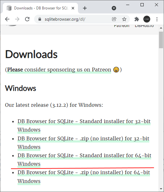
Например, в моем случае ОС — Windows 64x, поэтому я выбираю пакет DB Browser for SQLite — Standard installer for 64-bit Windows , который представляет установщик программы для 64-битной Windows.
После установки запустим программу:
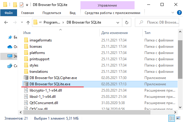
Нам откроется следующее окно
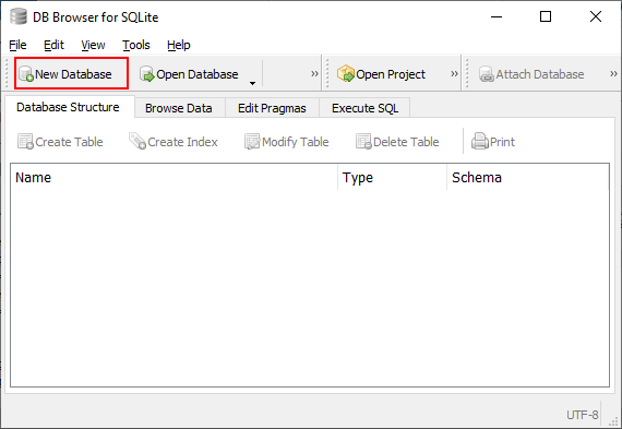
В рамках данной программы для управления базой данных мы можем использовать как графические возможности, так и запросы SQL. Так, создадим базу данных. Для этого нажмем на кнопку New Database (или через меню File -> New Database ). Далее нам будет предложено указать место и имя новой бд. Например, в моем случае файл базы данных будет называться people.db
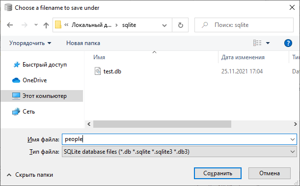
Впоследствии созданную базу данных можно будеть открыть с помощью кнопки Open Database или через меню File -> Open Database .
После этого нам будет предложено создать первую таблицу
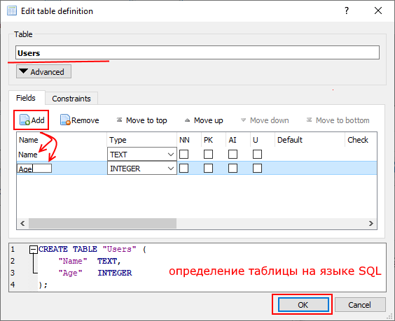
На этом окне в поле Table введем в качестве названия таблицы Users .
На вкладке Fields , которая содержит определения столбцов, нажмем на кнопку Add . И после нажатия в таблицу чуть ниже кнопки будут добавлять определения столбцов таблицы. Для первого столбца укажем в качестве имени Name , а в качестве типа — TEXT . Для второго столбца укажем в качестве имени Age , а в качестве типа — INTEGER .
То есть у нас будет таблица User со столбцами Name и Age.
После определения столбцов нажмем на кнопку OK, и программа сгенерирует новую таблицу:
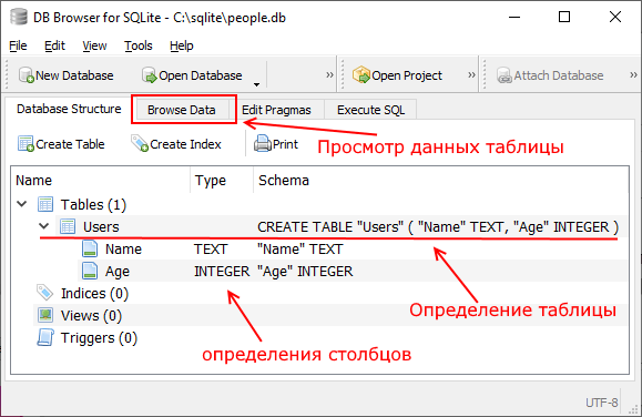
Для управления данными перейдем на вкладку Browse Data . По умолчанию у нас нет никаких данных
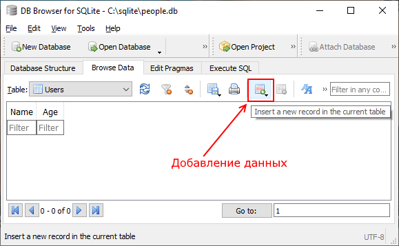
Добавим в таблицу одну строку. Для этого на панели инструментов нажмем на кнопку и в добаленную строку введем какие-нибудь данные:
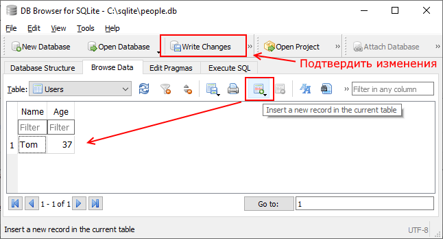
После добавления данных (впрочем как и после их изменения и удаления) для подтверждения изменений нажмем на панели инструментов на кнопку Write Changes (или на пункт меню File -> Write Changes ). И данные будут записаны в базу данных.
Выполнение запросов SQL
Также для упавления таблицами и данными можно использовать запросы SQL. Для написания и выполнения запроса SQL перейдем на вкладку Execute SQL
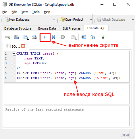
После этого в центральной части программы откроется окно для ввода скрипта SQL. Введем в него следующую команду:
Здесь создается таблица users2, которая фактически аналогична ранее созданной таблице users. Она также имеет два столбца name и age. И в нее добавляюся две строки.
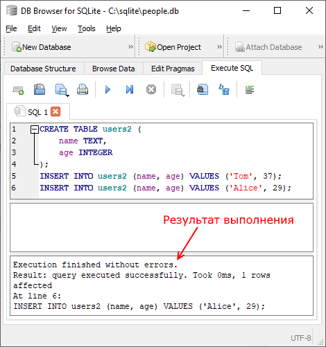
Для выполнения этого кода нажмем на синюю стрелку на панели инструментов. И после запуска кода SQL мы сможем увидеть отчет о его выполнения
После добавления мы можем получить данные. Для этого введем следующий код: